Part 1: install, extensions, virtual env.
Part 2: Initial Libraries and Data Import
Whew! Data is in, virtual environment is up, and we have executed some basic python commands.
Python is a great tool for exploring data, but if you are starting out it’s also another hurdle between you and the goal. This post will explore the Data Wrangler extension, introducing it as a part of your future workflow, where you can hopefully then expand your python skillset by proxy.
It’s not too late! Head back to the first post in the series so you can follow along.
From the official release page: '…Data Wrangler, a revolutionary tool for data scientists and analysts who work with tabular data in Python. Data Wrangler is an extension for VS Code and the first step towards our vision of simplifying and expediting the data preparation process on Microsoft platforms.
Data preparation, cleaning, and visualization is a time-consuming task for many data scientists, but with Data Wrangler we’ve developed a solution that simplifies this process. Our goal is to make this process more accessible and efficient for everyone, to free up your time to focus on other parts of the data science workflow. To try Data Wrangler today, go to the Extension Marketplace tab in VS Code and search for “Data Wrangler”. To learn more about Data Wrangler, check out the documentation here: GitHub - microsoft/vscode-data-wrangler '.
With Data Wrangler, Microsoft have developed an interactive UI that writes the code for you. As you inspect and visualize your Pandas dataframes using Data Wrangler, generating the code for your desired operations is easy. For instance, if you want to remove a column, you can right-click on the column heading and delete it, and Data Wrangler will generate the Python code to do that. If you want to remove rows containing missing values or substitute them with a computed default value, you can do that directly from the UI. If you want to reformat a categorical column by one-hot encoding it to make it suitable for machine learning algorithms, you can do so with a single command.
A great reference is this video from the Microsoft Data Wrangler team:
I would recommend the first 2 minutes if you don’t have long, however the summary of information in a little under 10 minutes is well worth the watch! You may recognise the data set
If you watched the video above, you will have seen a few different ways to explore the Titantic dataset. This is classic dataset, and whilst the I want to explore the contribution of different demographic values on the survival outcome of passengers.
Quick re-baseline steps:
reload VSCode
reopen the Folder (if needed - see blog 1)
load up the virtual environment (if needed - type .venv\scripts\activate - in the terminal.
With the python notebook open, you can open the dataframe in Data Wrangler via (1) Open short cut that appears at the bottom of the code block in the notebook - below:
The Data Wrangler window will open in a new tab. As you select different variables/fields you will see the data summary of each selected field calculated on the left (2) - screenshot below.
I prefer the descriptive statistics to be in a dedicated pane to the right in alignment with the video - you can emulate this by clicking on (1) ‘Toggle Secondary Side bar’ (Ctrl+Alt+B) in the image above. With the pane open, click and drag the data summary heading from the left pane to the right hand side. It should appear as per below:
Feel free to click around and explore. The blue button on the top right indicates we are in the Viewing mode, so we won’t be able to mess the data.
Clicking across the various fields I find the following three of interest:
Survival (numeric, 0% missing)
Sex (string, 0% missing)
SexCode (numeric, categorical, 0% missing)
Age (numeric, 42% missing)
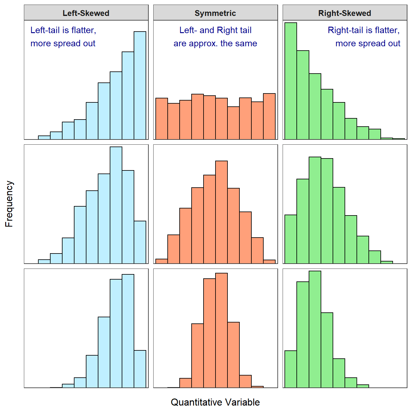
Age has the most interesting story here - lets note the distribution for now:
Visually we can see a skewed distribution - the right side tails off, flatter - this has a strong right skew.
For more on skewness there are a number of great resources - see the following:
Image from: https://derekogle.com/Book107/Book107_files/figure-html/ShapeExamples1-1.png
Module 5 Univariate EDA | Readings for MTH107 (derekogle.com)
Considering Age has 40% missing values, we would need to be careful with the management of missing values as it will likely cause a peak or potential bimodal distribution. We’ll come back to that!
One day Bing will learn to speel, today is not that day.
We’ve had an explore of the data, and currently my interest is around the following variables:
Survival (binary variable)
Gender (dichotomous variable)
Age (continuous variable)
Independent Variable (IV): A predictor or input variable that is used to determine the likelihood of a specific outcome in a given model.
Dependent Variable (DV): The outcome variable that the model aims to predict, indicating the direction, presence or absence of a particular event.
A short hand example of this concept, you could envision the above relationship as similar to DV = IVn+b. Don’t dwell on this, it’s not accurate for particular analyses, and I can feel my previous tutoring professors cringe from here.
I would like to explore Survival as the DV, with the IVs of Gender and Age, written as:
Probability of Survival as a product of Gender and Age.
As survival is a binary variable, gender is dichotomous and age is continuous - we need to use a Logistic Regression! Woo hoo!
Logistic regression is a statistical method used to model the relationship between a binary dependent variable and one or more independent variables. In the context of the Titanic dataset:
Dependent Variable (Survival): Indicates whether a passenger survived (1) or did not survive (0) the Titanic disaster.
Independent Variables (Predictors):
Gender: Categorical variable representing the passenger's gender (e.g., male or female).
Age: Continuous variable representing the passenger's age.
The logistic regression model can be used to predict the probability of a passenger's survival based on their gender and age.
For a logistic regression analysis, the data fields (variables) must meet certain requirements to ensure the model's validity and performance. Here are the key requirements and considerations for the data fields:
Dependent Variable:
Must be binary (i.e., takes on two possible outcomes, typically coded as 0 and 1).
Independent Variables:
Can be continuous, ordinal, or categorical.
Categorical variables must be converted to numerical codes or dummy variables (one-hot encoding).
Independence:
Observations should be independent of each other.
Logistic regression cannot handle missing values directly. Missing data must be addressed before fitting the model.
While the pandas library is essential for data manipulation and analysis, it does not provide functionality for performing logistic regression directly. To perform logistic regression in Python, you typically use the statsmodels or scikit-learn libraries. However, you can use pandas to prepare and manipulate your data before passing it to these libraries for the logistic regression analysis.
Logistic regression cannot handle missing values directly. We need to clean our missing values using Data Wrangler:
Survival (0% missing)
Sex (0% missing)
Age (42% missing)
There are different ways to reduce missing values. Due to the already low total case / row count, I’d like to avoid removing cases. Whilst contentious (and usually a much larger discussion) for this example lets replace missing values with appropriate values. The approach will be:
If a distribution is skewed, lets use the median value (The median value is the middle number in a sorted, ascending or descending, list of numbers, or the average of the two middle numbers when the list has an even number of observations)
If a distribution is normal, lets use mean (The mean value, or average, is the sum of all the numbers in a dataset divided by the total number of observation)
If a variable is categorical (i.e. survival) lets use the mode (The mode is the number that appears most frequently in a dataset)
As above the Logistic regression cannot handle missing values directly, so we need to clean our missing values using Data Wrangler! The missing values of Age, that is.
Earlier, we considered that Age has 40% missing values, so we need to be careful with the management of missing values as it will likely cause a peak or potential bimodal distribution - for this example we are going to use the median regardless.
Time to turn off the safety! Let move to editing mode in Data Wrangler by selecting (1) and (2) below:
Once you enter edit mode - a few things happen (screenshot below):
A Pop-up asks whether you want to open in Edit mode by default?
The left hand pane (where the descriptive statistics were earlier) now includes an operations menu.
With the descriptives safely out of the way on the right we are ready to work (almost like we planned it!).
Follow these steps to convert missing values of age to the median value:
Select Age
Select the Find and replace sub menu
Select Fill missing values
Select:
Fill Method
Median
See the preview of the resulting data change demonstrated in the green column to the right of the original Age field.
Have to say, I’m feeling less confident about the changes now. By changing the missing values to the median, we create an extreme artificial peak (1) - lets discard this change (2) and instead remove all cases with missing age.
On the operations menu, with age selected, select drop missing values. Observe the impact:
The distribution (obviously) represents the actuals.
The total case count has reduced from n=1310 to n=753.
The python code to make this change to the dataframe is presented in the preview pane.
We can apply the change by pressing apply.
Lets apply the change by pressing 4.
At the top of the screen select Export to notebook (1).
Back in the python notebook view, we now have a new code block generated by Data Wrangler. Run it.
Click the Data Wrangle open short cut to view the dataframe again - noting the file has n=753 rows. The drop of missing values worked and has been added to our code.
Add the following commands in an additional code block:
total_rows = len(dataframe_clean)
print(f"Total rows: {total_rows}")

unique_names_count = dataframe_clean['Name'].nunique()
print(f"Total unique names: {unique_names_count}")
Run the block.
Just double checking for consistency. Note the total count of rows differs from the count of unique name entries (the second code block) - due to file headers etc.
In this post we’ve explored the benefits of using Data Wrangler to explore our Titanic dataframe.
In the next post we will put it all together with a Logistic Regression via scikit-learn, documenting our findings via Markdown in the python notebook for practice.
See you soon wizards!
Continue to Part 4: Performing Logistic Recession on Target Data